Wetting, Drying, and Fluxes in SCHISM

Overview

Wetting and drying allows SCHISM to represent shorelines, tidal flats, levee slopes, and floodplains whose inundated area changes during a simulation. Understanding how SCHISM classifies nodes, elements, and sides is important when interpreting velocity, tracer transport, and the native flux.out diagnostic near a moving shoreline.

The key concept is that SCHISM does not impose a new hydrodynamic boundary condition along the instantaneous wet/dry front. Instead, it updates the wet/dry state of the fixed mesh as the shoreline moves. As a result, a side next to a dry element can remain hydrodynamically active even though tracer exchange across that side is suppressed. flux.out can also report a volume flux on such a side.

This page explains:

how the wet/dry state changes the active numerical domain
why hydrodynamic side flux and tracer exchange use different eligibility rules
how to interpret volume and tracer values in flux.out near a wet/dry front
why mesh resolution matters on banks and levee slopes

Wet/dry side states

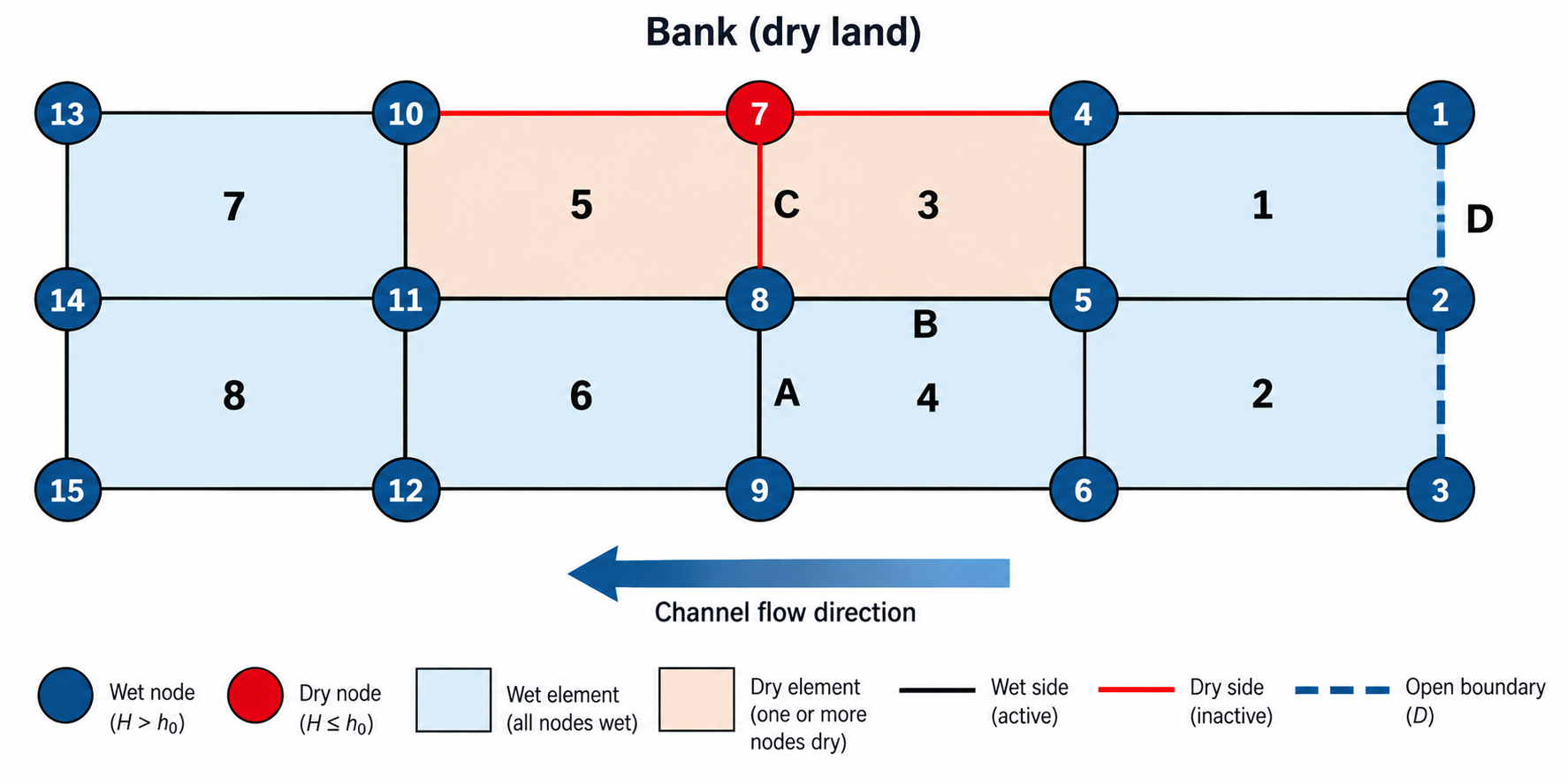
Fig. 15 Numbered schematic of a wet/dry bank transition and open boundary

The schematic represents a channel flowing from right to left, in the direction of the arrow. Node and element numbers increase downstream. Nodes are numbered down each cross-section before continuing to the next cross-section, and elements are numbered from the bank toward the channel bed before continuing downstream.

The northern edge is a bank. At node 7, the total water depth has fallen to or below the minimum depth threshold \(h_0\). An element is wet only when the total depth at every one of its nodes is greater than \(h_0\), so elements 3 and 5, which contain node 7, are dry in the state shown. SCHISM then derives the node and side states from the surrounding element states, as described in Wetting and drying changes mesh state. The figure shows three internal-side cases and one external-boundary case.

The labels are interpreted as follows:

A: the side from nodes 8 to 9, between wet elements 4 and 6
B: the side from nodes 5 to 8, between dry element 3 and wet element 4
C: the side from nodes 7 to 8, between dry elements 3 and 5
D: the open boundary along nodes 1, 2, and 3, adjoining wet elements 1 and 2

The three internal-side states are therefore

\[A:\text{wet/wet} \qquad B:\text{wet/dry} \qquad C:\text{dry}\]

These cases behave differently in the hydrodynamic solver, tracer solver, and flux diagnostic. The following sections use the lettered sides to connect each mesh state to its numerical behavior.

Wetting and drying changes mesh state

SCHISM begins the wet/dry classification by comparing the total depth at the nodes of each element with the specified minimum depth \(h_0\). The total depth is the water-surface elevation plus the bathymetric depth. The resulting states follow these rules:

an element is wet only if the total depth at all of its nodes is greater than \(h_0\); if any node is at or below the threshold, the element is dry
a node is wet if at least one surrounding element is wet; otherwise, it is dry
a side is wet if at least one adjacent element is wet; otherwise, it is dry

The classification therefore proceeds from the nodal depth test to the element state and then back to consistent node and side states. This is why side B in the schematic remains wet: it borders wet element 4. Side C is dry because both of its adjacent elements are dry.

SCHISM then carries wet/dry state through discrete flags used throughout the code, including element and side flags such as

idry_e
idry_s

The exact shoreline is therefore not represented as a continuously moving geometric boundary cutting arbitrarily through elements. Instead, the active numerical domain changes as node, element, and side states change.

This treatment differs from imposing a natural boundary condition.

At a true open model boundary, normal transport can enter the finite-element weak form through the boundary term. Schematically,

\[\int_\Omega \phi_i \nabla\cdot\mathbf U\,d\Omega = -\int_\Omega \nabla\phi_i\cdot\mathbf U\,d\Omega + \int_{\partial\Omega}\phi_i\,\mathbf U\cdot\mathbf n\,d\Gamma\]

A prescribed normal transport on a true external boundary therefore belongs naturally in the last term.

At the moving wet/dry front, however, SCHISM is not creating an internal boundary on which a new prescribed flux is imposed. Instead, it is changing which discrete nodes, elements, and sides are active.

For interpretation, treat the bank in the schematic as follows:

The shoreline is represented by changing state in the fixed mesh, not by imposing a special internal Neumann boundary condition that moves through the mesh.

Variable placement

The interpretation of sides B and C is easier once the staggering is remembered.

In SELFE/SCHISM:

free-surface elevation is stored at nodes
horizontal velocity is stored at side centers
tracer in the finite-volume formulation is associated with element/prism control volumes

Because the velocity degree of freedom lives on the side, a side can remain hydrodynamically active even when one neighboring element has become dry.

That is exactly the situation represented by B.

Case A: ordinary wet/wet side

Side A is the simple case.

Both adjacent elements are wet, and the side itself is wet. SCHISM therefore:

solves the side-centered horizontal velocity
constructs a normal volume flux from that velocity
allows the TVD tracer solver to exchange tracer between the two adjacent wet element control volumes
allows flux.out to integrate the side contribution when it lies on a specified flux-region interface

A layer contribution to volume flux has the form

\[Q_{A,k} = L_A \Delta z_k u_{n,A,k}\]

and the vertically integrated side flux is

\[Q_A = L_A\sum_k \Delta z_k u_{n,A,k}\]

Side A therefore represents ordinary interior transport between two active water volumes.

Case B: wet side with one dry neighbor

This case requires care when interpreting fluxes.

Assume

\[idry_s(B)=0\]

while one neighboring element is wet and the other is dry:

\[idry_e(E_{\rm wet})=0 \qquad idry_e(E_{\rm dry})=1\]

Hydrodynamics at B

The hydrodynamic code only zeros horizontal side velocity when the side itself is dry.

In schism_step(6).F90, the side loop contains the logic

if(idry_s(j)==1) then
  do k=1,nvrt
    su2(k,j)=0.d0
    sv2(k,j)=0.d0
  enddo
  cycle
endif

! Wet sides

So if B is a wet side, SCHISM continues into the hydrodynamic side calculation.

This means

\[\boxed{\mathbf u_B \text{ is an active hydrodynamic velocity degree of freedom}}\]

and it need not be zero.

The pressure-gradient reconstruction also treats the available wet neighboring element separately from a dry neighboring element. A wet/dry side is therefore not automatically shut down simply because one adjoining element is dry.

A geometric side-volume flux can consequently be formed:

\[Q_B = L_B\sum_k \Delta z_k u_{n,B,k}\]

This quantity can be nonzero.

Interpreting volume flux at B

A nonzero \(Q_B\) should not automatically be interpreted as

water is being conservatively transferred from the currently wet element into the currently dry element as though both were active finite-volume cells

That is not what the TVD tracer solver does.

The hydrodynamic side velocity and finite-volume tracer exchange have different eligibility rules.

Tracer transport at B

The explicit TVD transport routine first constructs horizontal advective water fluxes for wet sides.

In transport_TVD.F90.0, the side loop begins with

if(idry_s(j)==1) cycle

and then forms

flux_adv_hface(k,j)

from side-normal velocity multiplied by the vertical face area.

Thus a B-type side can have a defined hydrodynamic face flux in the transport routine.

However, when the tracer update loops around the faces of a wet element, it checks the neighboring element:

iel=ic3(j,i)

if(iel/=0) then
  if(idry_e(iel)==1) cycle
  trel_tmp_outside(:)=trel_tmp(:,k,iel)
...
endif

That cycle is decisive.

If the neighboring element is dry, the tracer solver skips that face before the inflow/outflow tracer update is applied.

Therefore, while the opposite element remains dry,

\[\boxed{\text{horizontal tracer exchange across B}=0}\]

There is not a one-sided operation in which the wet donor loses tracer mass while the dry receiver receives nothing.

In particular, SCHISM is not doing

\[M_{\rm wet}^{n+1} = M_{\rm wet}^n - Q_B C \Delta t\]

while simultaneously doing

\[M_{\rm dry}^{n+1} = M_{\rm dry}^n\]

That would be an obvious mass sink. The code avoids that by skipping the face in the tracer exchange when the neighboring element is dry.

The higher-order TVD limiter also explicitly requires two wet neighboring elements. Its logic skips a side when either neighboring element is dry.

So B is hydrodynamically active but is not an active wet-to-wet tracer exchange face.

WENO and implicit-vertical transport

The alternative transport implementation preserves the same horizontal wet/dry distinction. It uses implicit TVD in the vertical and explicit TVD in the horizontal. The WENO option (itr_met==4) changes the horizontal reconstruction, but when the neighboring element is dry the face is skipped before tracer exchange is performed.

For the explicit TVD, WENO, and implicit-vertical/TVD-horizontal paths, a B-type side can therefore retain a hydrodynamic face flux while horizontal tracer exchange with the dry neighboring element is omitted. Here, implicit describes the vertical treatment; it does not imply an implicit horizontal transfer across B.

Case C: dry side

Side C represents the stronger form of exclusion.

If

\[idry_s(C)=1\]

then the hydrodynamic side velocity is explicitly zeroed:

\[u_C=v_C=0\]

and the side is skipped in the relevant flux calculations.

So for C:

\[\boxed{\text{hydrodynamic side transport}=0}\]

\[\boxed{\text{TVD tracer exchange}=0}\]

\[\boxed{\text{native volume flux.out contribution}=0}\]

This is very different from B.

Case D: a true open boundary

Case D, shown at the right edge of the schematic, is a true model boundary. It is fundamentally different from either B or C.

For a prescribed-flow open boundary, SCHISM computes the wetted boundary cross-sectional area using wet boundary sides, and the prescribed transport is distributed over that area.

The code includes logic of the form

if(idry_s(isd0)==0) then
  carea = carea + htot*distj(isd0)
endif

and later, for prescribed flow,

vnth0=qthcon(ibnd)*ramp/carea(ibnd)

The corresponding normal velocity is imposed on the wet boundary sides.

Dry open-boundary sides are instead set to zero velocity.

This is the appropriate context in which to talk about an imposed normal-flow or natural boundary condition.

In short:

D is a boundary-condition problem. B and C are wet/dry-state problems.

Keep this distinction in mind when comparing prescribed boundary flow with fluxes near an inundation front.

How `flux.out` calculates volume flux

The native flux diagnostic in schism_step(6).F90 does not reconstruct a weak-form boundary term. It directly integrates solved side velocity over side area.

The relevant code excludes

if(idry_s(i)==1.or.isdel(2,i)==0) cycle

so it requires:

a wet side
an internal side with two mesh-neighbor element indices

It then forms the layer contribution

vnn=(su2(k+1,i)+su2(k,i))/2*snx(i)
   +(sv2(k+1,i)+sv2(k,i))/2*sny(i)

ftmp=fac*distj(i)*(zs(k+1,i)-zs(k,i))*vnn

which is simply

\[Q_k = L\,\Delta z_k\,u_{n,k}\]

The native volume diagnostic therefore measures a geometric transport associated with the solved side velocity.

Crucially, the code does not additionally require both neighboring elements to be wet.

Therefore:

\[\boxed{\text{A contributes to volume flux.out}}\]

\[\boxed{\text{B can contribute to volume flux.out}}\]

\[\boxed{\text{C does not contribute to volume flux.out}}\]

Consequently, a reported volume flux does not by itself establish that two wet tracer control volumes exchanged mass across the side.

10. Why B can appear in `flux.out` even though TVD tracer transport skips it

For a B-type side:

\[idry_s=0\]

so flux.out treats it as a wet internal side and integrates

\[Q_B=L_B\int u_{n,B}\,dz\]

But the tracer update asks an additional question:

Is the neighboring tracer control volume wet?

If the answer is no, it skips the exchange.

So the two operations answer different questions.

flux.out asks approximately:

What normal volume flux is implied by the solved velocity field on this wet side?

The tracer update asks:

Is there an active neighboring finite-volume tracer cell with which this wet cell can exchange tracer mass?

Those are not the same criterion.

This is why a nonzero flux.out value at a wet/dry interface should not automatically be interpreted as conservative exchange between two currently active water volumes.

11. Native tracer flux in `flux.out`

When tracer flux output is enabled, flux.out takes the same diagnostic water flux ftmp and multiplies it by an upwind element tracer concentration.

Schematically,

\[F_C^{\rm flux.out} = Q\,C_{\rm upwind}\]

The implementation uses the tracer value from one element when the side flux is positive and from the other when it is negative.

This is a diagnostic calculation.

It is not the same numerical operation as the prognostic TVD tracer update, which includes:

wet/dry control-volume eligibility
transport subcycling
TVD limiting where appropriate
diffusion
body-source terms
vertical fluxes
open-boundary tracer logic

The distinction becomes particularly important at B-type wet/dry interfaces because the diagnostic can still form \(Q C_{\rm upwind}\) even though the finite-volume tracer update skips wet-to-dry exchange across that face.

12. Rewetting and tracer state

The transport source contains the comment

For rewetted elements, tr_el takes the value from last wet step

This indicates that a newly rewetted element does not receive its initial concentration through a preceding B-face tracer transfer while it was still dry. Instead, its tracer state is restored from its previous wet state.

This is another reason to distinguish:

the hydrodynamic motion of the wet/dry front
the side-velocity-derived diagnostic flux
finite-volume tracer exchange between active wet cells
tracer state assigned when an element becomes wet again

The supplied source is sufficient to establish those separate code paths.

It is not sufficient, by itself, to prove an exact machine-precision global tracer-mass identity through every wet-to-dry and dry-to-wet state transition. A definitive proof of that would require tracing the routines that update the wet/dry masks and the element state during rewetting.

13. Unit-tracer thought experiment

A useful diagnostic is a conservative tracer initialized everywhere to

\[C=1\]

For an ordinary active wet/wet face,

\[F_C = Q C = Q\]

so the advective tracer flux and volume flux are numerically equivalent in units apart from the interpretation of the transported quantity.

At a B-type wet/dry face, however, the distinction becomes revealing:

a hydrodynamic side velocity can exist
flux.out can report \(Q_B\)
native diagnostic tracer flux can form \(Q_B C_{\rm upwind}\)
the tracer solvers examined here do not exchange tracer into the dry neighboring element

Thus even a unit tracer does not imply that every native side-flux diagnostic and every prognostic tracer transfer will match at the instantaneous wet/dry front.

The unit-tracer case is still useful because it removes concentration gradients from the problem and exposes the wet/dry bookkeeping directly.

14. Hydrodynamic conservation versus interpreting a single B-side flux

The original SELFE formulation emphasizes use of the primitive continuity equation and finite-volume definitions of volume when assessing conservation.

That should not be confused with the stronger claim that every nonzero side velocity at the edge of the active element set can be interpreted independently as conservative transfer into an active neighboring cell.

At B, the hydrodynamic solver carries a valid side velocity degree of freedom as part of the coupled free-surface and momentum solution. The complete hydrodynamic solution, moving free surface, vertical fluxes, and evolving wet/dry state determine the volume balance.

Therefore the safe interpretation is:

B has a real hydrodynamic velocity and a real velocity-derived geometric flux, but while the neighboring element is dry it is not an ordinary two-cell conservative tracer exchange face.

That statement is directly consistent with the source paths inspected here.

15. Why fine discretization on levee slopes remains important

The moving shoreline is represented discretely.

As water levels rise or fall, a node can change wet/dry state, which can in turn alter the state of neighboring elements and sides. On a coarse levee slope, one such transition can represent a relatively large change in:

horizontal shoreline position
elevation
active wetted area
storage volume
cross-sectional conveyance
which sides fall into A-, B-, or C-type behavior

With finer cross-slope resolution, these discrete transitions represent smaller physical increments.

A useful way to state the motivation is:

Fine discretization across wetting/drying slopes reduces the spatial, vertical, and cross-sectional quantization associated with discrete node, element, and side state changes as the shoreline migrates.

It also reduces the physical scale represented by B-type interface sides for which hydrodynamic velocity can remain active even though the neighboring tracer control volume is dry.

That provides a numerical reason, beyond simple bathymetric fidelity, for refining levee and bank slopes where wetting and drying is important.

16. Final interpretation table

Case	Mesh state	Hydr odynamic side velocity	G eometric side volume flux	TVD tracer exchange	Native volume `fl ux.out`	Inte rpret ation
A	wet side, we t/wet neig hbors	Yes	Yes	Yes	Yes	Ord inary int erior tran sport face
B	wet side, one wet and one dry nei ghbor	Yes	Pot entially n onzero	No while neighbor remains dry	Yes, if the di agnostic transect uses the side	A ctive hy drody namic side at m oving we t/dry front
C	dry side	No; zeroed	No	No	No	Ina ctive side
D	true ext ernal open bou ndary	Yes, a ccording to BC	Yes	B oundary- specific tracer t reatment	Separate boundary case	A ctual loc ation for im posed tr anspo rt/na tural BC

17. Final code-path table

Question	Hydrodynamics	TVD transport	`flux.out`
Is a dry side used?	No; velocity is zeroed	No	No
Can a wet side with one dry neighboring element remain active?	Yes	Face water flux can be formed, but horizontal tracer exchange is skipped	Yes
Are both neighboring elements required to be wet?	Not for the side velocity itself	Yes for the ordinary interior horizontal tracer exchange examined here	No
Is the quantity a prescribed we t/dry-interface boundary flux?	No	No	No
Can it represent a true imposed external flow BC?	Only at a true model boundary	Bo undary-specific treatment	Not the same operation
Is native tracer `flux.out` identical to prognostic TVD tracer transport?	—	—	No

Compact summary

For the four cases shown in the figure, the most concise interpretation is:

\[\boxed{ A:\ \text{hydro yes,\ tracer yes,\ flux.out yes} }\]

\[\boxed{ B:\ \text{hydro yes,\ tracer exchange no,\ flux.out yes} }\]

\[\boxed{ C:\ \text{hydro no,\ tracer no,\ flux.out no} }\]

The external case D is a true boundary-condition location:

\[\boxed{ D:\ \text{true boundary-condition location} }\]

The conceptual distinction to retain is:

The wet/dry front is represented by changing discrete state in the mesh. SCHISM is not imposing a moving internal natural boundary condition along that front.

19. Source basis

This note is based on the supplied files:

schism_step(6).F90
transport_TVD.F90.0
transport_TVD_imp.F90
Zhang and Baptista (2008), SELFE: A semi-implicit Eulerian–Lagrangian finite-element model for cross-scale ocean circulation
the supplied numbered A/B/C schematic (img/wet_dry_channel_example.png)

Relevant source locations inspected include:

schism_step(6).F90, approximately lines 6460–6650: wet-side momentum handling and zeroing of dry-side velocities
schism_step(6).F90, approximately lines 8965–9020: native flux.out calculation
schism_step(6).F90, approximately lines 2000–2100: open-boundary wetted-area and prescribed-flow logic
transport_TVD.F90.0, approximately lines 110–170: horizontal advective face-flux construction
transport_TVD.F90.0, approximately lines 295–335: requirement for two wet elements in the TVD limiter
transport_TVD.F90.0, approximately lines 850–970: actual horizontal tracer update and skip of dry neighboring elements
transport_TVD_imp.F90, opening comments: implicit TVD vertically and explicit TVD horizontally
transport_TVD_imp.F90, WENO branch near lines 270–730: WENO horizontal reconstruction and skip of a dry neighboring element
transport_TVD_imp.F90, later horizontal update near lines 1300–1330: dry-neighbor skip in the horizontal tracer update

One remaining source-level question, if a formal conservation audit is needed, is the exact sequence by which the current SCHISM version updates idry_e, idry_s, element volume, and restored tracer state during a wet/dry transition. The files examined here establish the side and transport behavior summarized above, but they do not by themselves provide the full mask-update routine needed for a complete proof of tracer-mass conservation through rewetting.