Gridding the Horizontal Mesh
The format of the SCHISM horizontal mesh is described in the SCHISM manual.
Users will find that SCHISM projects require refinement or extension. There are a few reasons:
SCHISM modeling is often used for
focused analysis, requiring refinement
sea level rise, requiring upstream extension or gridding of exposed areas.
restoration areas.
The spatial parameterization is varied or parameterized, so there is no extensive “calibration” of a new mesh
Here we will cover:
Best practices for horizontal gridding
Attaching boundaries
Checklist for after changing the grid or boundaries.
Vertical grid.
Meshing
Meshing considerations for SCHISM
Video (Joseph Zhang, SCHISM summit)
Video (Joseph Zhang #2)
Recap/checklist
Getting to know SMS
Please see Aquaveo SMS learning center for videos, tutorials, wiki, courses, and blog. The CA-DWR Delta Modeling Section has posted a series of videos to be used for learning how to use SMS for SCHISM mesh generation. You can see the complete playlist here: DMS SCHISM Gridding Playlist
Here’s the introductory SMS video by Eli Ateljevich:
Sample Data
Recap checklist
Presentation: clip_dems and efficient use of DEMS
Building the Bay-Delta mesh the standard way
Here’s the SMS 2dm generation overview video by Eli Ateljevich:
Presentation: Meshing consideration for marshes and restoration
Merging/Stitching SMS mesh/maps (new work, flooded islands, etc)
Video
Recap/checklist
Vertical mesh setup
Checklist for after you change the mesh
Changing the mesh tends to have consequences in places people forget to think about, though most are straightforward or obvious. This is a checklist of gotchas that arise outside the gridding environment.
☐ Are boundaries still in the proper place?
☐ If boundaries moved, is depth enforcement preventing dry boundaries still in right place?
☐ Are flow cross sections in changed area still aligned?
☐ Are the node pairs that define hydraulic structure locations still correct?
☐ Are polygons used to define spatial inputs appopriate for new area?
☐ If grid was extended, do yaml polygons cover extended domain?
☐ Are sources excluded?
☐ Do you have submerged aquatic vegetation? Assumptions? Consider changing those file
☐ Old hotstarts not valid on new mesh, utilities will interpolate on new grid
☐ Old nudging files not valid on new mesh. Re-do.
☐ If refining/coarsening extensively on main channel, consider the effect on momentum and the algorithm.
☐ Mesh quality:
☐ Skew and area warnings in preprocessor.
Performance Tuning
Changes in the horizontal mesh have the potential to create elements with small volume and fast velocities. Courant–Friedrichs–Lewy (CFL) condition for tracer transport will then trigger subcycling that will control the global performance of the model. Scaling and parallelism won’t help.
The first step in fixing this is to find the problem. The analyze_dt utility is intended to help diagnose which elements limit the global time step of the model. In pathological cases on a well-tended grid, a handful of elements are usually to blame. However, because a single bad element can control the time stepping of the entire model you do have to get them all.
Once you know identify bad actors, the following fixes may help:
Increase element size.
Add a small patch of emergent pseudo vegetation to create drag through the entire water column rather than shear from the bottom. Drag penalizes the square of velocity and will tap down flareups.
Coarsen the vertical mesh locally.
Convert triangles to quads.
Use elevation enforcement along the thalwag, which provides some smoothing.
The analyze_dt Utility
Note
To use this utility, you must run SCHISM with a build that includes the ANALYSIS module and ensure output for minTransportTimeStep is enabled in your model configuration (param.nml). The variable will appear in out2d_[#].nc
The analyze_dt utility is a subcommand within the bds command-line tool. It provides several tools to help identify and visualize elements in a SCHISM model domain that impose small transport time steps (minTransportTimeStep) during simulations. This is useful for debugging and mesh refinement, especially where subcycling might be triggered.
This utility is available as a subcommand:
bds analyze_dt [COMMAND] [OPTIONS]
Available Commands
- dist
Plot a cumulative distribution function (CDF) of time steps.
Example:
bds analyze_dt dist out2d_21.nc --file_step 5- hist
Plot a histogram focusing on the lower end of time steps.
Example:
bds analyze_dt hist out2d_21.nc --file_step 5- list
List the N elements with the smallest time steps at a given output step within the file.
Example:
bds analyze_dt list out2d_21.nc --file_step 3 --n 20Sample Output:
ndx,el,x,y,dt
0,315764,595402.84,4226879.11,1.731465
1,310596,595791.67,4225754.48,1.749715
...
- plot
Plot the spatial distribution of transport time steps, highlighting the lowest N.
Example:
bds analyze_dt plot out2d_21.nc --file_step 2 --n 20- summarize
Analyze and optionally plot elements that frequently appear among the lowest N time steps across all output times.
Options:
summarize: Top N elements to track each timestep
–num: Minimum number of appearances required to be included
–plot: Flag to show a spatial plot
–csv_out FILE: Save results to CSV
–label_top K: Label top K offenders (default: all)
Example:
bds analyze_dt summarize out2d_21.nc --summarize 20 --num 10 --plot --csv_out dt_summary.csv
This example summarizes elements that appear among the 20 worst offenders per time step for at least 10 time steps. The output includes the (0-based) element number, count of times in this role and location.
Sample Text Output:
el,count,x,y
3363,31,652052.58,4172820.80
310595,31,595791.67,4225754.48
...
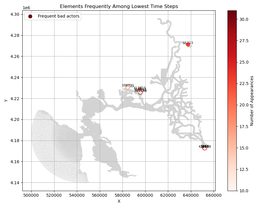
Fig. 14 Figure Example plot of 20 elements with smallest subcycling time steps