Module 6: Overview

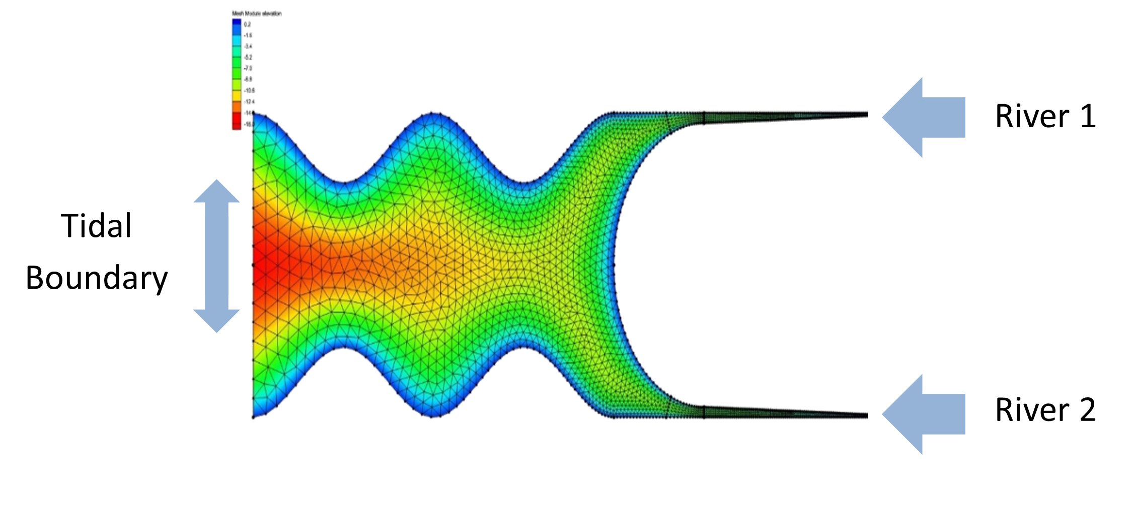
In this module we will modify the three open boundaries applied to the model domain as seen in Fig. 10. The directory for this module is “./modules/m6_boundaries”.

Fig. 10 Simplified domain used for Hello SCHISM practice problems. Ocean boundary is on the left, two river inputs on the right. Domain length in the x direction is roughly 56km

Note

The boundaries are pre-defined in the hgrid.gr3 file which was created with prepare_schism (see Module 2: Preprocessor for more info).

Salinity Boundaries

Barotropic v. Baroclinic

This module is building off of the base “Hello SCHISM” set-up (See Module 1: Hello SCHISM). In the base setup salinity is resolved (modeled as a tracer) and the model is ran in three dimensions. Because the model resolves salinity, density-driven circulations can be represented and thus the setup is “baroclinic” as opposed to “barotropic” - where density is dimensionally uniform.

For this exercise we will create a barotropic simulation.

1. Open the file “./modules/m6_boundaries/param.nml”

• Search for iof_hydro(19) and set this to 0. This will turn off salinity output.

2. Open the file “./modules/m6_boundaries/bctides.in”

   The current setup for River 1 looks as follows:

   4 0 2 0 2 0 ! River 1: 4 nodes wide, elevation (0=unspecified), flow (1=*.th time history, 2=constant), temperature (0=unspecified), salinity (2=constant), generic tracer ()
   -20.0      ! Constant inflow
   4.0        ! Constant salt
   1.0        ! Salt nudging
   

   The first line means:

   4	0	2	0	2	0
   Number of nodes in BC	Elevation definition (0=unspecified, 1=*.th time history file, 2=constant, 3=tidal amplitude/phases, …)	Flow definition (0=unspecified, 1=*.th time history file, 2=constant, 3=tidal amplitude/phases, …)	Temperature (0=unspecified, 1=*.th time history file, 2=constant, 3=relax to init. cond., …)	Salinity (0=unspecified, 1=*.th time history file, 2=constant, 3=relax to init. cond., …)	Generic Tracer (0=unspecified, 1=*.th time history file, 2=constant, 3=relax to init. cond., …)

   Then the following lines specify the constant flow, salinity, and salt nudging factor as -20.0, 4.0, and 1.0, respectively.

3. Remove salinity from this boundary by changing the fifth entry (2) to a 0, and deleting the lines which define the constant salinity (4.0) and salt nudging factor (1.0).

4. Repeat step 3 with River 2.

5. With the ocean boundary the values are similar to that of the rivers, but now the values will look like:

   17 3 0 0 2 0 ! Ocean: 17 nodes, type of boundary (3=tidal constituents), elev and temp not specified, constant salt
   Z0
      1.000000000000000        0.0000000000000
      1.000000000000000        0.0000000000000
   ...
   

   The first line means:

   17	3	0	0	2	0
   Number of nodes in BC	Elevation definition (0=unspecified, 1=*.th time history file, 2=constant, 3=tidal amplitude/phases, …)	Flow definition (0=unspecified, 1=*.th time history file, 2=constant, 3=tidal amplitude/phases, …)	Temperature (0=unspecified, 1=*.th time history file, 2=constant, 3=relax to init. cond., …)	Salinity (0=unspecified, 1=*.th time history file, 2=constant, 3=relax to init. cond., …)	Generic Tracer (0=unspecified, 1=*.th time history file, 2=constant, 3=relax to init. cond., …)

   To remove salinity from this boundary change the fifth entry (2) to 0 and remove the lines at the bottom of the file that specify the constant salinity (12.0) and salt nudging factor (1.0).

   6. Save the file

Now you have made the necessary edits to the bctides.in and param.nml files for the run to be barotropic in that there is no account for spatially-varying water density.

Stage Time Series at Ocean Boundary

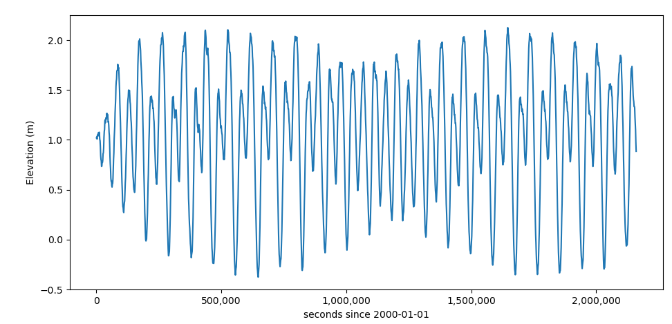
Currently, the ocean boundary in the model uses tidal harmonic constituents (eg: M2, O1, K1) to define the open stage boundary. If, instead, you wanted to define the boundary with a time series, you can use a file with a “.th” extension. The file is provided in the “./modules/m6_boundaries” directory and is called “elev.th”.

Fig. 11 Time series plot of the elev.th file

1. Open the bctides.in file you modified earlier

2. Navigate to the line that contains “! Ocean: 17 nodes” and change the second entry (3) to 1. This means that the model will use a time history file called “elev.th”

3. Save the file

Now SCHISM will see that the ocean elevation boundary requires a “elev.th” ascii file to specify the stage at the boundary in seconds since the reference model time.

River Inflow Boundaries

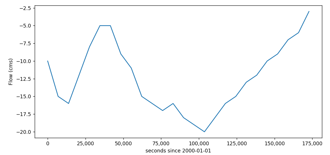
As mentioned before, the two rivers use a constant inflow boundary of -20 cms (cubic meters per second). We are now going to change the inflow for River 1 to be a time-varying inflow.

Fig. 12 Time series plot of the flux.th file

Note

The flow applied to the boundary is negative if entering the model domain.

1. Open the bctides.in file you modified twice now

2. Navigate to the line that contains “! River 1” and change the third entry (2) to 1. Now the model will point to a time history file called “flux.th”. Delete the line specifying the constant flow of -20.0 cms.

3. Save the file. Now SCHISM will see that the River 1 boundary requires a “flux.th” ascii file to specify the stage at the boundary in seconds since the reference model time.