Timeseries operations and function¶

VTools provides a number of time series operations and functions.

Python Imports¶

A lot of the functions are split off in their own files. If you are writing a module for reuse, you may want to use the modules and do a minimal import for name hiding. However, for analysis everything in the functions API can be accessed using this import:

from vtools.functions.api import *

Interpolation¶

There are several vtools functions for interpolation. Your choice of function and interpolation method should hinge on:

whether you are interpolating to a new set of times or filling gaps

to interpolate to new times (perhaps using another time series as a prototype): interpolate_ts()

to fill gaps: interpolate_ts_nan()

whether your time series is instantaneous or period averaged:

Most methods assume instantaneous. Use the function rhistinterp() for period averaged data or the RHIST method option from the abovementioned functions. The

tension parameter can also be used to enforce a lower bound (e.g. positivity of salinity).

The interpolation method will depend on:

how smooth the series is:

LINEAR is robust in noisy data

MSPLINE is a monotonicity preserving spline that combines great accuracy with good robustness.

SPLINE is the spline technique from Scipy which is a smoothing spline, not an exact interpolant. The spline is slower than the others.

RHIST is the best choice for period averaged data

PREVIOUS means the previous value will be repeated. Good for discrete valued data such as gate opening and closing.

NEXT means the forward value will be copied backward.

whether you need an “exact” interpolant that goes through all values exactly.

whether you need to enforce monotonicity or positivity. If these are important, MSPLINE and RHIST are preferred.

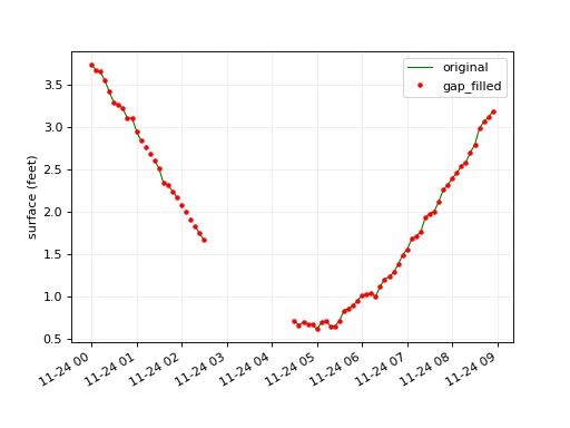
Here is an example of how inteprolate_ts_nan() fills nan values on an existing series. : and inteprolate_ts() which interpolates one time series to a new interval or to times from a sample series or time sequence.

"""Examples of performing interplation over time
   series.
"""

## load necessary libs.
from vtools.functions.interpolate import *
from vtools.data.sample_series import *
import matplotlib.pyplot as plt


ts_with_nan=example_data("pt_reyes_tidal_with_gaps")
## fill the invalid (nan) data points within a time
## series by linear interpolation.
ts_new=interpolate_ts_nan(ts_with_nan,method=LINEAR,max_gap=4)

fig=plt.figure()
ax0 = fig.add_subplot(111)
ax0.set_ylabel("surface (feet)")
p0=ax0.plot(ts_with_nan.times,ts_with_nan.data,color='g',linewidth=1.,)
p1=ax0.plot(ts_new.times,ts_new.data,color='r',linestyle="none",marker=".")
plt.legend(["original","gap_filled"])
plt.grid(b=True, which='major', color='0.9', linestyle='-', linewidth=0.5)
fig.autofmt_xdate()
plt.show()

(Source code, png, hires.png, pdf)

Low Pass Filtering (noise, tidal, spring-neap)¶

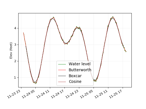
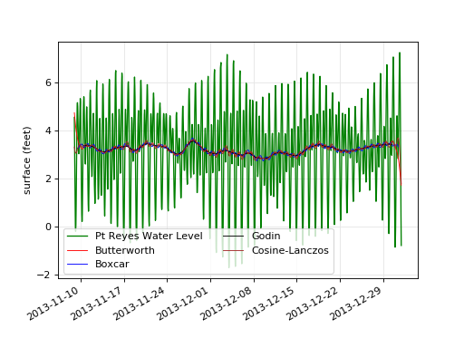
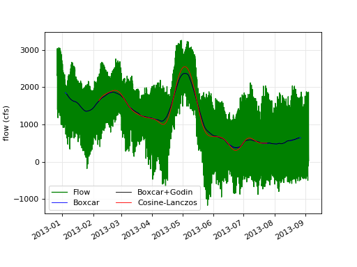
The cases below are all just special cases of low pass filtering, but motivated by different goals (noise removal, tidal filtering and spring-neap filtering). All of the filters are phase-neutral, meaning they do not cause an apparent shift in the time series as a single pass of a Cosine-Lanczos or Butterworth filter might do.

For tidal filtering, we recommend the cosine-Lanczos (really CL squared) filter with a cutoff of 40 hours which is fairly standard in the tidal literature. The Godin filter is commonly used for its simplicity and minimal support which means less amplification of gaps. However, its performance on signals with a period of 2-3 days is abysmal.

Noise filter¶

from vtools.functions.filter import *
from vtools.data.sample_series import *

import matplotlib.pyplot as plt

## 1 day of tide at point reyes
ts_1day=example_data("pt_reyes_tidal_6min")
ts_butt=butterworth(ts_1day,cutoff_period="1hour")
boxcar_aver_interval = parse_interval("1hour")
ts_box=boxcar(ts_1day,boxcar_aver_interval,boxcar_aver_interval)
ts_cos=cosine_lanczos(ts_1day,cutoff_period=hours(1),filter_len=10)
fig=plt.figure()
ax0 = fig.add_subplot(111)
ax0.set_ylabel("Elev (feet)")
lwidth=0.8
p0=ax0.plot(ts_1day.times,ts_1day.data,color='green',\
            linewidth=lwidth,label="Water level")
p1=ax0.plot(ts_butt.times,ts_butt.data,color='red',\
            linewidth=lwidth,label="Butterworth")
p2=ax0.plot(ts_box.times,ts_box.data,color='black',\
            linewidth=lwidth,label="Boxcar")
p3=ax0.plot(ts_cos.times,ts_cos.data,color='brown',\
            linewidth=lwidth,label="Cosine")
plt.legend(loc="lower center",prop={'size':12})
plt.grid(b=True, which='major', color='0.9', linestyle='-', linewidth=0.5)
fig.autofmt_xdate()
plt.show()

(Source code, png, hires.png, pdf)

Tidal filter¶

# -*- coding: utf-8 -*-


from vtools.functions.filter import *
from vtools.data.sample_series import *
import matplotlib.pyplot as plt
import datetime

ts=example_data("pt_reyes_tidal_1hour")
## only plot part of result
window_start=datetime.datetime(2013,11,25)
window_end=datetime.datetime(2013,12,2)
ts_cosine=cosine_lanczos(ts,cutoff_period=hours(30),filter_len=30,padtype="constant")
#ts_cosine=temp.window(window_start,window_end)
ts_butt=butterworth(ts,cutoff_period=hours(60),order=4)
#ts_butt=temp.window(window_start,window_end)
boxcar_aver_interval = hours(12)
ts_box=boxcar(ts,boxcar_aver_interval,boxcar_aver_interval)
#ts_box=temp.window(window_start,window_end)
ts_god=godin(ts)
#ts_god=temp.window(window_start,window_end)
fig=plt.figure()
ax0 = fig.add_subplot(111)
ax0.set_ylabel("surface (feet)")
#ts=ts.window(window_start,window_end)
lwidth=0.8
p0=ax0.plot(ts.times,ts.data,color='green',\
           linewidth=1.2,label="Pt Reyes Water Level")
p1=ax0.plot(ts_butt.times,ts_butt.data,color='red',\
           linewidth=lwidth,label="Butterworth")
p2=ax0.plot(ts_box.times,ts_box.data,color='blue',\
           linewidth=lwidth,label="Boxcar")
p3=ax0.plot(ts_god.times,ts_god.data,color='black',\
           linewidth=lwidth,label="Godin")
p4=ax0.plot(ts_cosine.times,ts_cosine.data,color='brown',\
           linewidth=lwidth,label="Cosine-Lanczos")
plt.grid(b=True, which='both', color='0.9', linestyle='-', linewidth=lwidth)
plt.legend(loc="lower left",ncol=2)
fig.autofmt_xdate()
plt.show()

(Source code, png, hires.png, pdf)

Spring-neap filter¶

# -*- coding: utf-8 -*-
from vtools.functions.filter import *
from vtools.data.sample_series import *
import matplotlib.pyplot as plt
import datetime as dtm

window=(dtm.datetime(2012,12,27),None)
ts=example_data("oldriver_flow").window(*window)
ts_lowpass=cosine_lanczos(ts,cutoff_period=days(18),filter_len=2000)
boxcar_aver_interval = days(8)
ts_box=boxcar(ts,boxcar_aver_interval,boxcar_aver_interval)
ts_box_god=godin(ts_box)
fig=plt.figure()
ax0 = fig.add_subplot(111)
ax0.set_ylabel("flow (cfs)")
lwidth=0.8
p0=ax0.plot(ts.times,ts.data,color='green',linewidth=1.2,label="Flow")
p2=ax0.plot(ts_box.times,ts_box.data,color='blue',\
            linewidth=lwidth,label="Boxcar")
p3=ax0.plot(ts_box_god.times,ts_box_god.data,color='black',\
            linewidth=lwidth,label="Boxcar+Godin")
p4=ax0.plot(ts_lowpass.times,ts_lowpass.data,color='red',\
            linewidth=lwidth,label="Cosine-Lanczos")
plt.grid(b=True, which='both', color='0.9', linestyle='-', linewidth=lwidth)
plt.legend(loc="lower left",ncol=2)
fig.autofmt_xdate()
plt.show()

(Source code, png, hires.png, pdf)

Resampling and decimation¶

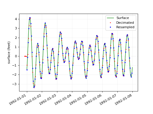
vtools.functions.resample() takes a finer time series and downsamples it to a coarser time step. vtools.functions.decimate() is a refimenment of this strategy which first passes the data through a low pass filter then resamples. Our version comes from a GNU Octave .m function. Decimation is also something you can do yourself. Just low pass to a period twice that of the time step you want to resample at. So if you are going to resample at a one hour frequency, eliminate everything with a period short of two hours.

# -*- coding: utf-8 -*-

from vtools.functions.resample import *
from vtools.data.sample_series import *
import matplotlib.pyplot as plt


ts=synthetic_tide_series()
ts_decimate=decimate(ts,hours(1))
ts_resample=resample(ts,hours(1))
fig=plt.figure()
ax0 = fig.add_subplot(111)
ax0.set_ylabel("surface (feet)")
p0=ax0.plot(ts.times,ts.data,color='g',linewidth=1.2)
p1=ax0.plot(ts_decimate.times,ts_decimate.data,color='r',\
marker=".",linestyle="none",markersize=3)
p2=ax0.plot(ts_resample.times,ts_resample.data,\
color='b',marker="*",linestyle="none",markersize=3)
plt.legend(["Surface","Decimated","Resampled"])
plt.grid(b=True, which='major', color='0.9', linestyle='-', linewidth=0.5)
fig.autofmt_xdate()
plt.show()

(Source code, png, hires.png, pdf)

Ufuncs on time series¶

OK, not a very informative name but ufuncs (universal functions) are a standard numpy method for applying the same function to every item in one or two time series. Furthermore, the operation can be done cumulatively or pointwise. See the .. _numpy ufunc docs: http://docs.scipy.org/doc/numpy/reference/ufuncs.html. These documents give a good descripation of what the apply, reduce and accumulate methods do.

In vtools, ufuncs are supported in the vtools.functions.ts_ufunc module(). The ufunc is pretty much passed right over to the data member of the time series, so this is just a convenience. The generic implementations for time series are ts_apply() ts_accumulate() and ts_reduce(). There are also some specific ufunc implementations for time series such as ts_maximum() that are potentially useful.

Period ops¶

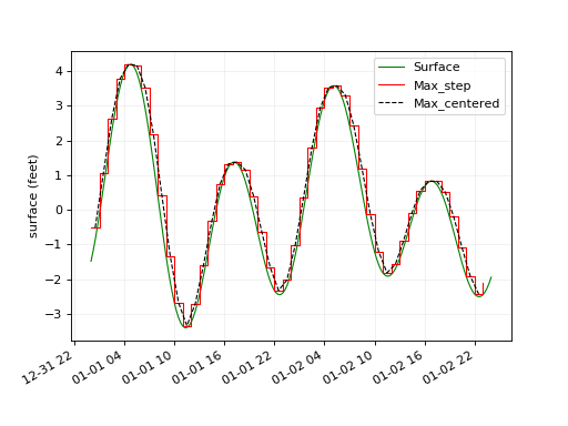
VTools provides for creating period statistics such as daily/monthly averages, max or min. The output of these operations is a new time series at a coarser time step.

# -*- coding: utf-8 -*-

from vtools.functions.period_op import *
from vtools.data.vtime import days
from vtools.data.sample_series import *
import matplotlib.pyplot as plt


ts_week=synthetic_tide_series()
## get 2 days of data
ts=ts_week.window(ts_week.times[0],ts_week.times[0]+days(2))
ts_max=period_max(ts,hours(1))
fig=plt.figure()
ax0 = fig.add_subplot(111)
ax0.set_ylabel("surface (feet)")
p0=ax0.plot(ts.times,ts.data,color='g',linewidth=1.0)
p1=ax0.step(ts_max.times,ts_max.data,color='r',linewidth=1.0,where="post")
p2=ax0.plot(ts_max.centered().times,ts_max.centered().data,color='black',\
linewidth=1.0,linestyle="--")
plt.legend(["Surface","Max_step","Max_centered"])
plt.grid(b=True, which='major', color='0.9', linestyle='-', linewidth=0.5)
fig.autofmt_xdate()
plt.show()

(Source code, png, hires.png, pdf)

Shifting¶

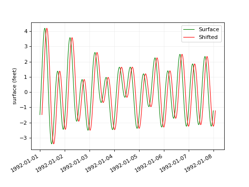
Time series can be shifted forward or back in time with vtools.functions.shift().

# -*- coding: utf-8 -*-

from vtools.functions.shift import *
from vtools.data.sample_series import *
from vtools.data.vtime import hours
import matplotlib.pyplot as plt


ts=synthetic_tide_series()
ts_shifted=shift(ts, hours(2))
fig=plt.figure()
ax0 = fig.add_subplot(111)
ax0.set_ylabel("surface (feet)")
p0=ax0.plot(ts.times,ts.data,color='g',linewidth=1.0)
p1=ax0.plot(ts_shifted.times,ts_shifted.data,color='r',linewidth=1.0)
plt.legend(["Surface","Shifted"])
plt.grid(b=True, which='major', color='0.9', linestyle='-', linewidth=0.5)
fig.autofmt_xdate()
plt.show()

(Source code, png, hires.png, pdf)

Merging¶

VTools will facilitate a prioritized merging using vtools.functions.merge():

from vtools.functions.api import merge
ts_merged = merge(ts_high_priority,ts_medium,ts_low)

Table Of Contents

Previous topic

Next topic

This Page

Timeseries operations and function¶

Python Imports¶

Interpolation¶

Low Pass Filtering (noise, tidal, spring-neap)¶

Noise filter¶

Tidal filter¶

Spring-neap filter¶

Resampling and decimation¶

Ufuncs on time series¶

Period ops¶

Shifting¶

Merging¶